


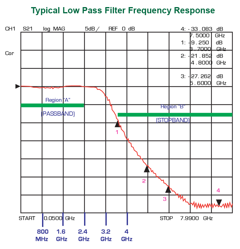
The graph shown here illustrates a typical low pass filter (LPF) function. It indicates how much attenuation is achieved at a given frequency for, in this instance, the IMF2293. All other LPF graphs will be similar to this one, but will have different frequency spans and different gradients depending on the design of the filter.
In order to quote/specify a low pass filter, the following information must typically be provided:
1. The extent of the passband (i.e.; what frequencies does the low pass filter PASS?).
2. The passband insertion loss (how much power is dissipated by the filter).
3. The stop band attenuation levels and frequencies (which frequencies does the filter reject and by how much?).
Generally, IMS filters will have passband insertion losses ranging between 0.5 dB and 1.0 dB with a few exceptions, depending on design. If a customer needs less than 0.3dB loss, it is unlikely that IMS can meet that requirement. Conversely, if the customer can live with greater than 2 dB insertion loss, then they may be able to use an off the shelf low cost LTCC device. The extent of the passband is usually described as “DC to 1.5GHz” or “DC to 2.4GHz” or “DC to some frequency” (region “A” on the graph, see reverse side).
Sometimes, a customer will simply describe the passband as a single frequency (DC is implied), e.g., a “2.5 GHZ low pass filter” because their transmitter or receiver is working at 2.5GHZ.
A low pass filter designed for this purpose would be exactly the same as a LPF that would be designed for someone who requests “DC to 2.5 GHZ”.
It should be noted that most transmitters cannot work at more than a small band of frequencies anyway, but this does not change the design of a low pass filter, nor does it change the need for a low pass filter in a system.
The stopband (region “B” in the graph) attenuation (also referred to as “rejection”) is the most important aspect of a low pass filter’s function. Usually, an engineer will say “I need a 2.5GHZ low pass that has 20 dB of rejection at the 2nd and 3rd harmonics”. What this means is that his passband is approximately (or ends at) 2.5 GHz and that he needs 20 dB of attenuation at 5 GHz (the 2nd harmonic of 2.5 GHz) and also 20 dB of rejection at 7.5GHz (the 3rd harmonic).
Most implementations of a low pass filter are to suppress harmonics but not always. A key point is to make certain that what is specified is the stopband frequencies (harmonic or not) and also to specify the rejection needed at those frequencies.
Note on the picture that the filter response shows a passband that ends between approximately 2.4GHz and 3.2 GHz (it was designed for 2.4GHz). Note also that marker 2 identifies the 2nd harmonic (2 X 2.4GHz = 4.8 GHz) and additionally depicts a rejection level (attenuation) of 21.8dB at 4.8GHz.
Generally speaking, the more rejection an engineer needs at a given frequency, the more sections in a filter that are necessary. This makes the filter longer, which also contributes to a higher insertion loss as well as more real estate. There are techniques available that can be used in some cases to minimize size, dependent on the individual application.
If the frequency at which rejection is needed is closer to the passband than 2f (the 2nd harmonic frequency), then more sections may be needed in a filter for a given level of attenuation. For instance, if filter “A” needs 30 dB of rejection at 5GHz while filter “B” needs 30 dB of rejection at 4GHz (and both their passbands end at 2.5 GHz), then it is likely that more sections are needed for filter “B”.
VSWR is largely unimportant to specifying a LPF, because the measure of VSWR is primarily dependent on how the customer mounts the filter and to what it is being mounted. At IMS, all LPF’s are designed with an assumed VSWR of 1.1:1 (which equates to 25 dB return loss) unless it is necessary to relax the VSWR spec in order to achieve a higher rejection for a given filter. The assumption is that the part will be mounted in a matched 50 ohm system whose material constants are the same as that of the filter itself; an ideal situation. All filters have input and output connections that are 50 ohm impedance unless otherwise specified.
Basically, VSWR, rejection and insertion loss (and thus power level) all play against one another in any filter design. This makes filters a challenge to design, and also underscores the importance of providing accurate and detailed information to the supplier in order to accurately specify, design, and quote them.
Take a look at IMS’ low pass planar filters.
Download our tech note here.